Implementing Keyframe Animation

In this post I will show you the way I implemented a keyframe-based 3D real time animation using WebGL. Familiarity with the WebGL / OpenGL rendering pipeline, and with linear algebra is necessary. There don't seem to be many well-made explainations online about real time 3D animation with WebGL which aren't involving Three.js and COLLADA so I hope that this will be useful for those who wish to program their own animations.

We will model a mesh in Blender (a bit of familiarity is necessary here, too), rig it up, write a barebone set of shaders and boilerplate code from scratch, and then load, parse and run the animation in our WebGL context.

You can download all the materials for this tutorial here, or view them on GitHub here.

Keyframe based animation is one of the most known algorithms for animating 3D models, another very important one being skeletal animation / mesh skinning / rigging (or countless other names I've read it described as). Like all algorithms, it has upsides and downsides. Keyframe based animation consists of "taking snapshots" of the animated model at different points in time, which could be as many or as few as needed, and to render those frames one after the other. Optionally, you could linearly interpolate (lerp) the geometry between keyframes in order to have a smoother transition.

Skeletal animation expands the concept by implementing keyframe animation on a quite smaller mesh, which is called a rig or an armature. The vertices of the rig, and their transformation matrix, control each one a subset of the vertices of the main, bigger mesh, partially or totally, depending on a weight that each vertex of the main mesh has defined for each vertex of the rig. More concepts are involved, such as Inverse Kinematics and bone parenting, but we will discuss those in another post dedicated specifically to skeletal animation.

Let's now look at when and why to use keyframe based animation.

The good

Keyframe based animation is useful when you can't (or don't want to) put too much pressure on the computation power of your GPU. Keyframes are created as Vertex Buffer Objects and the only operation required to switch between frames is to set the proper VBOs before a drawElements call, allowing you to write light-weight shader code.

The bad

Keyframe based animation takes a LOT of VBO space. A simple, bare bone mesh like the one in this tutorial takes ~400kb for a handful of frames. Most of the time this isn't the case and your animation may get to various megabytes in a horribly fast manner, since we are cloning each vertex and each normal countless times. Also this isn't really physics-engine friendly because the code knows really nothing about the mesh, so it must use every vertex to do the calculations. Not cool. Skeletal animation is way more suited for situations like this one.

The ugly

Caution is advised, be mindful of where and why you are implementing this algorithm. In this tutorial we're going to use the Wavefront OBJ format for its simplicity but you'll want to find another format to hold your data, be it a roll-your-own JSON structure, COLLADA, FBX or whatever it is you are most comfortable working with. We're gonna cover WebGL but this really can be done in any language that supports an OpenGL-like rendering pipeline.

Okay, let's get to it!

Part 1: Modeling and rigging

We will use Blender for this purpose. At the time of writing, version 2.70a is out. We will create a complete, usable (albeit very minimal) model of a barb-like thingamabob that bends itself towards the ground. The screenshots are downloadable in a higher resolution along with the rest of the code and the .blend file.

First of all, we will want to create a geometry like the one portrayed in Step 01. The way I did this was by extruding three times the upper face of a unit cube so that I had three connected cubes, one on top of each other, then I loop-selected (Alt + right click) the edges of the horizontal faces and scaled them to smaller values from bottom to top. Specifically I kept the lowermost face intact, scaled the next one to 0.75, the next one to 0.5 and the topmost to 0.0 - getting four vertices collapsed in the same spot, making a pyramid.

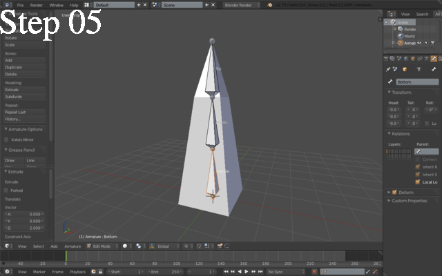
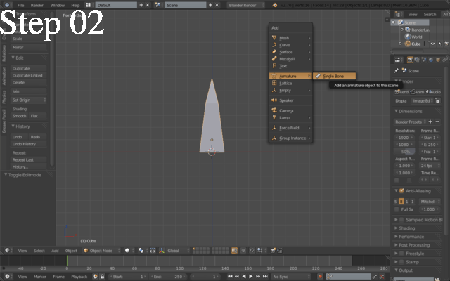
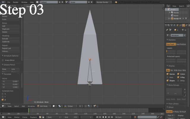
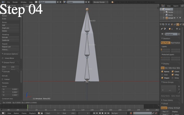
Next thing you want to do is to create an armature (see Step 02). Make sure your 3D cursor is at the bottom-center of the mesh, select Add > Armature > Single bone. Position the bone as shown in Step 03 and then, keeping the upper joint (the little sphere) selected, extrude it twice and position the bones as seen in Step 04. Also, make sure the "Names" and "X-Ray" checkboxes are checked in the Display properties of the armature (see the panel on the right side) to help yourself with positioning. Rename then each of the three bones; you should now have something similar to Step 05

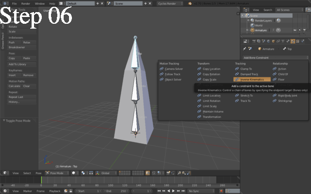
Let's then add an Inverse Kinematic constraint to our rig. Right click the armature, enter Pose Mode, select the topmost bone and add a constraint as shown in Step 06.

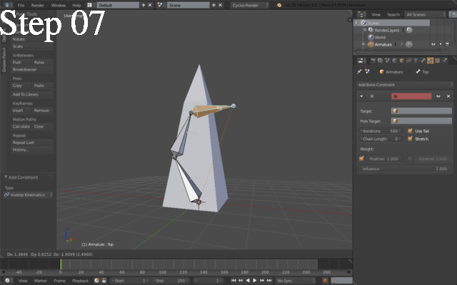
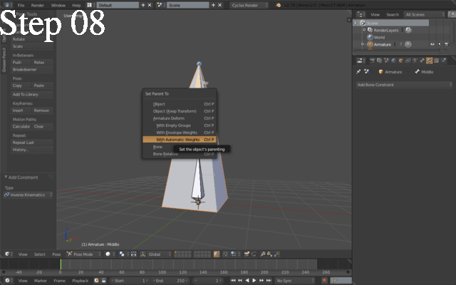
Step 07 shows the constrained armature bending. We then proceed to parent the mesh to the armature by first selecting the mesh, then shift-selecting the armature (Shift + right click), then pressing Ctrl+P to bring out the parenting menu, and then selecting Armature deform - with automatic weights (Step 08).

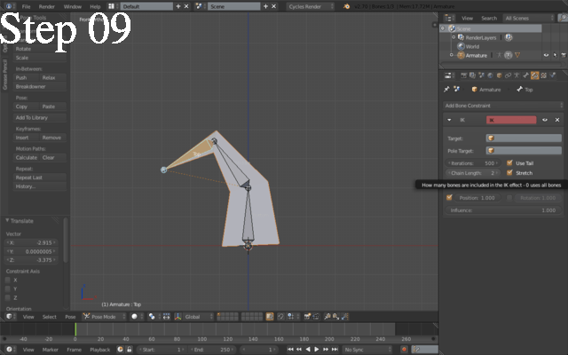
We must now set the chain length of the inverse kinematic constraint to 2; this will limit its influence to the top and middle bones, so the bottom one can stay put while the other two bend towards the ground, to obtain the effect seen in Step 09.

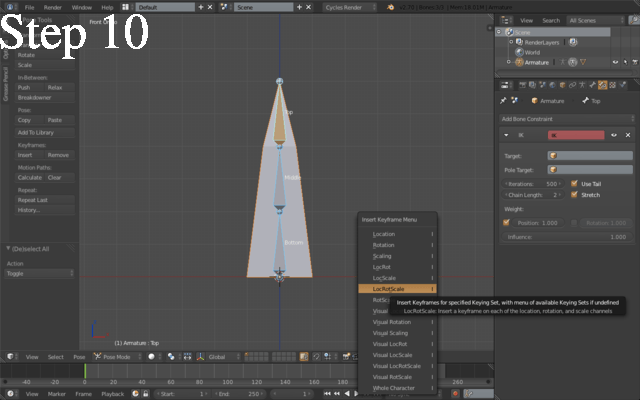
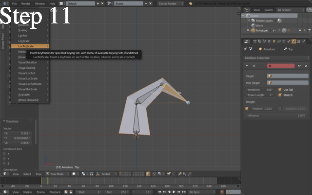
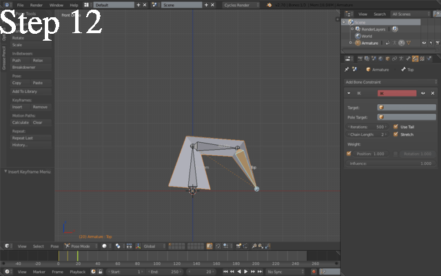
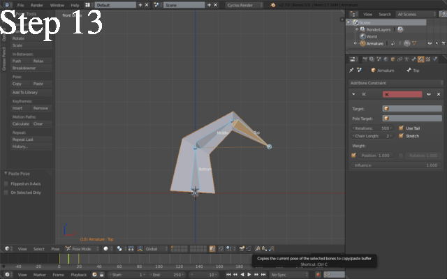
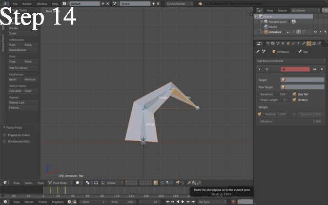
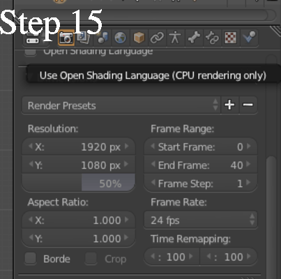
Now is the time to animate our armature. Let's keyframe the neutral position at frame 0 by selecting the whole armature in Pose Mode, pressing I in the 3D view and choosing LocRotScale (Step 10). Let's then bend a little bit the topmost bone and repeat the keyframing, twice, at frames 10 and 20 (Steps 11, 12). To make the animation symmetric, copy and paste the pose at frame 10 on frame 30, and the pose at frame 0 on frame 40, as shown in Steps 13 and 14. Set the start frame to 0 and the end frame to 40 as shown in Step 15.

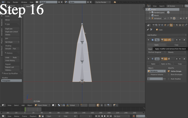
IMPORTANT STEP, DO NOT SKIP. Add a Triangulate faces modifier to the mesh, move it on top of the armature modifier and apply it immediately. This will allow us to export coherent animation frames, because Blender's OBJ exporter's "triangulate" option causes a bit of trouble (Step 16).

You will also want to UV Unwrap the mesh, so that the texture mapping is included in the exported file. This is important if you are going to use the parser included in the download code, since it doesn't handle missing texture coordinates. At last, export as OBJ file; it is important that the options are coherent with what is shown in Step 17, for the same reason (poorly written parser).

Yay, we made it!

Part 2: Animating the model in WebGL

2.1 Boilerplate

First of all, let's get the boilerplate code out of the way. We will use no external libraries besides gl-matrix. We will use a barebone flat shader program, reported below:

// Vertex shader - vertex.glsl
uniform mat4 uP, uV, uM;
uniform mat3 uN;

attribute vec3 aVertex, aNormal;
attribute vec2 aTexCoord;

varying vec3 vVertex, vNormal;

void main() {

  gl_Position = uP * uV * uM * vec4(aVertex, 1.0);
  vVertex = aVertex;
  vNormal = aNormal;

}

// Fragment shader - fragment.glsl
precision highp float;

uniform mat4 uP, uV, uM;
uniform mat3 uN;

uniform sampler2D uSampler;
varying vec3 vVertex, vNormal;

void main() {

  vec3 lAmbient = vec3(1.0, 1.0, 1.0);
  vec3 lDiffuse = vec3(0.5, 0.5, 1.0);
  vec3 lSpecular= vec3(1.0, 1.0, 1.0);

  vec3 plPos = vec3(0.0, 3.0, 5.0);
  vec3 plDir = normalize(plPos - vVertex);

  mat4 mvp = uP * uV * uM;
  vec3 n = normalize(uN * vNormal);
  vec3 l = normalize(vec3(mvp * vec4(plDir, 1.0)));
  vec3 v = normalize(-vec3(mvp * vec4(vVertex, 1.0)));
  vec3 r = reflect(l, n);

  float lambert = dot(l, n),
        ambientInt = 0.2,
        specularInt = 0.5,
        diffuseInt = 1.0,
        shininess = 128.0;

  float specular = pow( max( 0.0, dot(r,v) ), shininess );

  gl_FragColor = vec4(
      lAmbient * ambientInt +
      lDiffuse * diffuseInt * lambert +
      lSpecular * specularInt * specular
      , 1.0);
}

We will then want to initialize our WebGL context, load and compile our shader program and make the uniforms' and attributes' locations available to the "outside". For simplicity, we are loading the shaders via a synchronous XMLHttpRequest so we don't get caught up in callbacks and promises. Clearly, those are things that should be addressed in production code because it is unacceptable to make the user wait with the browser idle while the assets are loaded, but this is not the main focus of the post.

// Initialize WebGL context
var gl = (function() {

  var canvas = document.getElementById('canvas');
  canvas.style.position = 'fixed';

  var gl = canvas.getContext('webgl') ||
           canvas.getContext('experimental-webgl') ||
           console.log('WebGL unsupported');

  canvas.width = window.innerWidth;
  canvas.height = window.innerHeight;

  gl.viewport(0, 0, canvas.width, canvas.height);

  window.addEventListener('resize', function() {
    canvas.width = window.innerWidth;
    canvas.height = window.innerHeight;

    gl.viewport(0, 0, canvas.width, canvas.height);

  });

  return gl;

}());

// Compile the shader program, pack the uniform locations in it and
// return the whole thing
var prog = (function(gl, attribs, uniforms) {

  var compileShader = function(source, type) {
    var xhr = new XMLHttpRequest();
    xhr.open('GET', source, false);
    xhr.send();

    var shader = gl.createShader(type);
    gl.shaderSource(shader, xhr.responseText);
    gl.compileShader(shader);
    console.log('Shader compilation:', gl.getShaderInfoLog(shader));

    return shader;
  }

  var program = gl.createProgram();
  gl.attachShader(program,
                  compileShader('vertex.glsl', gl.VERTEX_SHADER));
  gl.attachShader(program,
                  compileShader('fragment.glsl', gl.FRAGMENT_SHADER));

  gl.linkProgram(program);
  gl.useProgram(program);

  for(var i in attribs)
    program[attribs[i]] = gl.getAttribLocation(program, attribs[i]);

  for(var i in uniforms)
    program[uniforms[i]] = gl.getUniformLocation(program, uniforms[i]);

  return program;

}(
  gl,
  ['aVertex', 'aNormal'],
  ['uM', 'uV', 'uP', 'uN']
));

Let's abstract the logic behind the construction and drawing process of a mesh. We create a Mesh object whose constructor takes a geometry layout (vertices, indices, normals and other information) and creates buffers in GPU memory space that will contain the data. It is mostly a matter of createBuffer, bindBuffer and bufferData calls.

var Mesh = function(geometry) {
  this.geometry = geometry;

  this.vertexBuffer  = gl.createBuffer();
  this.indexBuffer   = gl.createBuffer();
  this.normalBuffer  = gl.createBuffer();

  gl.bindBuffer(gl.ARRAY_BUFFER, this.vertexBuffer);
  gl.bufferData(gl.ARRAY_BUFFER,
                new Float32Array(this.geometry.vertices),
                gl.STATIC_DRAW
               );
  gl.bindBuffer(gl.ARRAY_BUFFER, this.normalBuffer);
  gl.bufferData(gl.ARRAY_BUFFER,
                new Float32Array(this.geometry.normals),
                gl.STATIC_DRAW
               );
  gl.bindBuffer(gl.ELEMENT_ARRAY_BUFFER, this.indexBuffer);
  gl.bufferData(gl.ELEMENT_ARRAY_BUFFER,
                new Uint16Array(this.geometry.indices),
                gl.STATIC_DRAW
               );

  gl.bindBuffer(gl.ARRAY_BUFFER, null);
  gl.bindBuffer(gl.ELEMENT_ARRAY_BUFFER, null);
}

The geometry object will also hold spatial information that will allow us to construct the model matrix (uM in the shaders). This information is position, rotation and scale and we will use the excellent gl-matrix library to calculate the matrix at each draw call. We will also calculate the normal matrix (uN), needed for the lighting algorithm, as the inverse transpose of the model matrix. Then we will bind the matrices to the corresponding uniforms, bind the buffers to the attributes, issue a call to drawElements and unbind the buffers until the next call.

Mesh.prototype.draw = function(baseMatrix) {
  var mvMatrix = mat4.create();
  var nMatrix  = mat3.create();

  if(typeof baseMatrix !== 'undefined') {
    mvMatrix = mat4.clone(baseMatrix);
  } else {
    mat4.identity(mvMatrix);
    mat4.translate(mvMatrix, mvMatrix, this.geometry.position);
    mat4.rotate(mvMatrix, mvMatrix,
                this.geometry.rotate[0], [1.0, 0.0, 0.0]);
    mat4.rotate(mvMatrix, mvMatrix,
                this.geometry.rotate[1], [0.0, 1.0, 0.0]);
    mat4.rotate(mvMatrix, mvMatrix,
                this.geometry.rotate[2], [0.0, 0.0, 1.0]);
    mat4.scale(mvMatrix, mvMatrix,
               this.geometry.scale || [0.6, 0.6, 0.6]);
  }

  mat3.normalFromMat4(nMatrix, mvMatrix);

  gl.uniformMatrix4fv(program.uM, false, mvMatrix);
  gl.uniformMatrix3fv(program.uN, false, nMatrix);

  gl.bindBuffer(gl.ARRAY_BUFFER, this.vertexBuffer);
  gl.vertexAttribPointer(program.aVertex, 3, gl.FLOAT, false, 0, 0);
  gl.enableVertexAttribArray(program.aVertex);

  gl.bindBuffer(gl.ARRAY_BUFFER, this.normalBuffer);
  gl.vertexAttribPointer(program.aNormal, 3, gl.FLOAT, false, 0, 0);
  gl.enableVertexAttribArray(program.aNormal);

  gl.bindBuffer(gl.ELEMENT_ARRAY_BUFFER, this.indexBuffer);

  gl.drawElements(this.geometry.rendering,
                  this.geometry.indices.length,
                  gl.UNSIGNED_SHORT, 0
                 );

  gl.bindBuffer(gl.ARRAY_BUFFER, null);
  gl.bindBuffer(gl.ELEMENT_ARRAY_BUFFER, null);
}

We will now prep the animation loop. What we want to do is to initialize the perspective and view matrix. gl-matrix comes to our help with the function mat4.perspective for the former, and we perform a simple translation from the identity matrix for the latter. We then set the GL context's clear color to black and enable the depth testing.

var uP = mat4.create(), uV = mat4.create();
mat4.perspective(uP, 45,
                 window.innerWidth / window.innerHeight,
                 0.01, 500.0
                );
mat4.identity(uV);
mat4.translate(uV, uV, [0, -2, -10.0]);

gl.clearColor(0.0, 0.0, 0.0, 1.0);
gl.enable(gl.DEPTH_TEST);

We will have an array of meshes that will constitute our animation frames, so we create a simple requestAnimationFrame-based drawing loop that increments a counter by a time-dependent amount, so that we end up having the same animation speed no matter what the frame rate is. The counter is, clearly, a floating point value; we cast it to integer and reduce modulo the number of frames so an infinite animation loop is performed. Don't be afraid if some variables seem uninitialized; they are defined earlier in the code, in a part we will discuss soon.

var curMesh = 0, curMeshf = 0.0;

(function animate(time) {

  var delta = time - (animate.timeOld || time);

  gl.clear(gl.COLOR_BUFFER_BIT | gl.DEPTH_BUFFER_BIT);

  gl.uniformMatrix4fv(prog.uP, false, uP);
  gl.uniformMatrix4fv(prog.uV, false, uV);

  if(meshes.length > 0 && meshes[curMesh] !== undefined) {
    // Rotate the mesh around the Y axis
    meshes[0].geometry.rotate[1] += 0.02;
    meshes[curMesh].draw();
  }

  if(meshes.length > 0) {
    if(!isNaN(delta)) curMeshf += 0.05 * delta;
    curMesh = parseInt(curMeshf);
    curMesh %= meshes.length;
  }

  requestAnimationFrame(animate);
  animate.timeOld = time;

}(0));

We now need some code to parse our Wavefront OBJ files. I found this nice tutorial that explains the ins and outs of the format using C++ syntax. If you made it this far, I am confident you can get the gist of it even if you don't know C++. Anyway here's the parsing code. We first read all the lines, parsing the vertices, normals and texture coordinates, then we parse the faces and adapt them to GL's standard - which is indices. We then build the vertices, indices, normals and texc (texture coordinates; present although not used here) arrays and return them as our geometry layout object.

function parseObj(t) {
  var vertices = [], fverts = [], indices = [],
      normals = [], fnormals = [], flist = [],
      texc = [], ftexc = [];

  for(var i = 0; i < t.length; i++) {
    var line = t[i], m = null;

    if(m = line.match(/^v ([^\s]+)\s([^\s]+)\s([^\s]+)/)) {
      fverts.push(parseFloat(m[1]));
      fverts.push(parseFloat(m[2]));
      fverts.push(parseFloat(m[3]));
    } else if(m = line.match(/^vn ([^\s]+)\s([^\s]+)\s([^\s]+)/)) {
      fnormals.push(parseFloat(m[1]));
      fnormals.push(parseFloat(m[2]));
      fnormals.push(parseFloat(m[3]));
    } else if(m = line.match(/^vt ([^\s]+)\s+([^\s]+)/)) {
      ftexc.push(parseFloat(m[1]));
      ftexc.push(parseFloat(m[2]));
    } else if(m = line.match(/^f (\d+)\/(\d*)\/(\d+)\s+(\d+)\/(\d*)\/(\d+)\s+(\d+)\/(\d*)\/(\d+)/)) {
      var i1 = m[1], i2 = m[4], i3 = m[7],
          n1 = m[3], n2 = m[6], n3 = m[9],
          f1 = m[2], f2 = m[5], f3 = m[8];

      i1--; i2--; i3--;
      n1--; n2--; n3--;
      f1--; f2--; f3--;
      flist.push([i1, n1, f1]);
      flist.push([i2, n2, f2]);
      flist.push([i3, n3, f3]);

    }

  }

  for(var i = 0; i < flist.length; i++) {
    var f = flist[i];
    indices.push(i);
    vertices.push(fverts[f[0] * 3]);
    vertices.push(fverts[f[0] * 3 + 1]);
    vertices.push(fverts[f[0] * 3 + 2]);
    normals.push(fnormals[f[1] * 3]);
    normals.push(fnormals[f[1] * 3 + 1]);
    normals.push(fnormals[f[1] * 3 + 2]);
    texc.push(ftexc[f[2] * 2]);
    texc.push(ftexc[f[2] * 2 + 1]);
  }

  return {
    vertices: vertices,
    normals: normals,
    indices: indices,
    textureCoordinates: texc // unused here
  };
}

2.2 Keyframe animation, at last!

Boilerplate code is finally over! Let's see how we can load, parse and animate our model.

We have a couple of options here. If you recall, we keyframed our rigged model at keyframes 0, 10, 20, 30 and 40, and Blender exported 40 .obj files for us. In this case we might be fine, but if the geometry was just a tiny little bit more complicated than that we'd be in for some pain. I designed a model for a project of mine which is a bit more complex but still very low poly, and with just a couple more keyframes than this I found myself with 10 megabytes worth of files for a legs-only animation. Unacceptable, considering the simplicity.

If we don't mind employing a little GPU buffer space (and we don't mind, do we?), we may resort to a different solution that is a nice middle ground between loading times and algorithmic load. We will just make use of a bunch of the exported frames, namely the keyframes - which, by themselves, could not make for a nice and smooth animation - and calculate the frames in between (tween) via linear interpolation.

Linear interpolation (lerp for the buddies) is a formula that calculates an intermediate point between two numbers, or vector, or matrices. This point is calculated as if it were on a line (hence the linear part). We can find as many or as few intermediate points as we need, but we must supply a parameter that will tell us how far or how close we are to one of the two points. This parameter ranges from 0.0 to 1.0 where 0.0 means "exactly the first point", 1.0 means "exactly the second point", 0.5 means "exactly in the middle of the two", you get the idea. So for example if we need ten intermediate frames, we shall make ten linear interpolations at ten equally spaced points between two frames. This means pushing a frame on the stack, sampling between the first and second keyframe at 0.1, then at 0.2, ... then at 0.9, then taking the final point and pushing it onto the stack with the other frames - or sampling another at 1.0, which is the same thing. Then we repeat the process by interpolating between the former "second keyframe" and the next keyframe at the same points 0.1 - 1.0 as before; notice that we skip sampling at 0.0 except for the first time, since we already have on stack the frame corresponding to the new frame interpolated at 0.0. Also, the last keyframe we stop interpolating at 0.9 since the sample at 1.0 would be the same as the absolute first frame we pushed.

So this is how we do it: we pick four keyframes (the first and the last will be one and the same, so we leave out the fifth), we load them synchronously via XMLHttpRequest, we parse them, we interpolate 10 frames, get 10 geometries, create a Mesh for each of those and push it onto the meshes array. The XHRs are synchronous for the same reason I explained earlier, plus for the fact that we need each frame to arrive at the exact same moment we need it, or we risk getting the order wrong.

// objFile holds the four keyframes we're going to use
var meshes = [], objFiles = [
  "skeletal_000000.obj",
  "skeletal_000010.obj",
  "skeletal_000020.obj",
  "skeletal_000030.obj"
];

for(var i = 0; i < objFiles.length; i++) (function(obj, i) {

  // XHRs are sync here because we must push the meshes in the correct
  // order. It's okay here because we don't need anything fancy but
  // you should never do this in the real world and opt for a correct
  // asynchronous behaviour, but this is not the place to discuss it.
  var xhr = new XMLHttpRequest();
  xhr.open('GET', 'frames/' + obj, false);
  xhr.onreadystatechange = function() {
    if(this.readyState !== 4) return;

    var t = this.response.split('\n');
    var geom = parseObj(t); // parse file
    geom.rendering = gl.TRIANGLES;

    if(meshes.length > 0) {
      // If this is not the first object, then the pos/rot/scale should
      // all reference the pos/rot/scale on the very first mesh, so
      // we can alter these and the changes will propagate through the
      // meshes. There are way better ways to do this, but still
      geom.position = meshes[0].geometry.position;
      geom.rotate = meshes[0].geometry.rotate;
      geom.scale = meshes[0].geometry.scale;

      // Pick the last geometry from the previous iteration
      var prevGeom = meshes[meshes.length - 1].geometry;
      // Get ten geometries linearly interpolated (lerped) between
      // the current and the previous keyframes
      for(var k = 1; k < 10; k++) {
        var lg = lerpGeometry(prevGeom, geom, k/10);
        meshes.push(new Mesh(lg));
      }

    } else {
      geom.position = [0.0, 0.0, 0.0];
      geom.rotate = [0.0, 0.0, 0.0];
      geom.scale = [1.0, 1.0, 1.0];
      meshes.push(new Mesh(geom));
    }

    // Finally, lerp last and first keyframe to get a
    // seamless animation
    if(i == objFiles.length - 1) for(var k = 0; k < 10; k++) {
      var lg = lerpGeometry(geom, meshes[0].geometry, k/10);
      meshes.push(new Mesh(lg));
    }
  }
  xhr.send();

}(objFiles[i], i));

The LERPing operation itself is quite simple. We initialize a new object with the properties of the first keyframe, replace the vertices, indices and normals with fresh, new empty arrays, and fill them up with the interpolated values. Actually, filling up the indices array wouldn't be necessary since we know the order is the same in each keyframe, we could cut it out for added performance and space saved; creating new vertices and normals array is important, though.

function lerpGeometry(a, b, t) {

  var out = {}, i;

  // Copy non strictly geometry-related properties in the output.
  // This is specific to the format used in this code and may or
  // may not be useful in other contexts.
  for(i in a) if(a.hasOwnProperty(i)) out[i] = a[i];

  // Assign new, empty arrays to our geometric properties
  out.vertices = [];
  out.indices = [];
  out.normals = [];

  // Loop through the indices "just like" the GL pipeline would
  for(i = 0; i < a.indices.length; i++) {
    // Current index. Same index should match the same vertices on
    // both a and b geometries
    var index = a.indices[i];

    // Push the index as-is
    out.indices.push(a.indices[i]);

    // Lerp the vertices. Take (1-t) % from a, (t) % from b.
    // Note that t should always be between 0 and 1
    out.vertices.push(
      // X component
      a.vertices[index * 3] * (1 - t) +
      b.vertices[index * 3] * t,

      // Y component
      a.vertices[index * 3 + 1] * (1 - t) +
      b.vertices[index * 3 + 1] * t,

      // Z component
      a.vertices[index * 3 + 2] * (1 - t) +
      b.vertices[index * 3 + 2] * t
    );

    // Lerp the normal. Same as the vertex
    out.normals.push(
      a.normals[index * 3] * (1 - t) +
      b.normals[index * 3] * t,

      a.normals[index * 3 + 1] * (1 - t) +
      b.normals[index * 3 + 1] * t,

      a.normals[index * 3 + 2] * (1 - t) +
      b.normals[index * 3 + 2] * t
    );
  }

  return out;
}

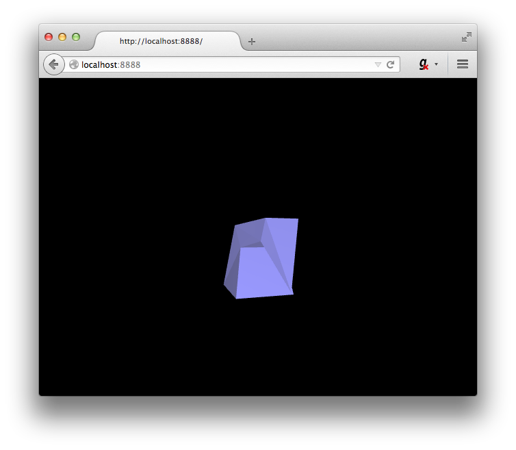
So here's our final result. If you have any questions, please feel free to ask in the comments and I will gladly integrate anything missing or useful. Again, to get the code of the tutorial along with the pre-exported OBJs and Blender file, click here, or click here to view them directly on GitHub. Hope you enjoyed!